ACI Topology and Hardware
ACI Hardware
Though this chapter is called ACI Topology and Hardware we begin with the hardware. This makes more sense from a logical standpoint. Otherwise I would be telling you about Leafs and Spines and APICs and such, without any reference.
There is a lot of specific hardware available for ACI and I won’t cover it all here. The best place to find hardware specific information is on the Cisco website itself. ACI uses Cisco Nexus 9000 series switches, more specifically the 9500 series and the 9300 series. Most of these switches can be implemented as ‘regular’ NX-OS switches too.
Cisco has created a taxonomy that they use to name the switches. This taxonomy is relevant for anybody working with Nexus 9000 series switches and people working with ACI. Of course the taxonomy can change, so check the following page for the most recent information: Taxonomy for Cisco Nexus 9000 Series
The naming uses the following logic:
N9K-ZYYXXXWV-U where:
- Z = Platform type
- C means a switch or Chassis
- X means a line card
- YY = Platform Hardware
- 93 = Fixed port (ToR) NX-OS or ACI switch
- 95 = Modular Chassis
- 97 = NX-OS or ACI line card
- XXX = The bandwidth of all the ports in 10’s of Gbps, or if all ports are the same, the number of ports
- W = Type of downlink ports (max speed and type of interface)
- G = 100/1000Mbit copper
- Y = 25Gbit SFP
- C = 100Gbit QSFP28
- V = Uplink type (Same codes as downlink types)
- U = Special capabilities
- F = MacSec
- E = Enhanced ACI
- X = Analytics, Netflow and Microsegmentation
The above list is incomplete, but includes the most important information for ACI networks. For a complete list look at the Taxonomy link above.
For example the Cisco Nexus N9K-C93180YC-EX switch, which is currently a very common switch in ACI deployments can be explained as follows:
- It is a fixed port switch
- It has 1800Gbps of bandwidth
- It has 25Gbps SFP downlink ports
- It has 100Gbps QSPF28 uplink ports
- It has Enhanced ACI and Analytics support
Spine switches
Spine switches are special switches that provide the backbone of the ACI fabric. All Leaf switches must connect to the spines and the spines take care of the leaf to leaf traffic. Spine switches often contain a lot of 40 or 100Gbit/s ports. These ports provide the required bandwidth for the ACI fabric.
In the first iteration of ACI you could only connect Leafs to a Spine. But as ACI evolved, some options for connecting other devices to Spine switches came available. The most common ones are Multi-Pod and Multi-Site (more on which later), but there are others. Endpoints are still only allowed on Leaf switches though.
Leaf switches
What then are Leaf switches? Leafs are the switches in ACI to which all endpoints, interconnects and services connect. There is a plethora of possible Leaf switches available with port speeds ranging from 100/1000Mbps to 400Gbps (which will soon be available) and with or without FC(oE) support. This diverse offering makes it possible for each customer to select the correct switches to fit their needs.
Leaf switches are often categorized by function:
- Border Leaf: These switches are used to connect external networks to the fabric
- Service Leaf: Services like loadbalancing and firewalls are often connected to these Leafs
- Compute Leaf: These leafs are used to connect regular endpoints, and can be called regular leafs as well
- Transit Leaf: The transit leaf is a special role that exists in stretched fabric topologies only. These are the leafs that connect to the spines in other datacenters.
When building a large fabric it might make sense to split the above functions. But, many fabrics aren’t big enough to dedicate special leaf (pairs, as leafs are often configured in pairs) to these functions. If you have two outside connections from the fabric it doesn’t make sense to sacrifice 46 out of the 48 ports on a switch purely to have a dedicated border leaf. Because of that all of the above roles can be combined as you see fit.
APICs
The APICs are the controllers for ACI. APIC stands for Application Policy Infrastructure Controller. This is the central point of management for the ACI fabric. On the APIC an administrator creates a policy which will in turn be translated into configuration by the APIC. This configuration is then pushed into the right switches.
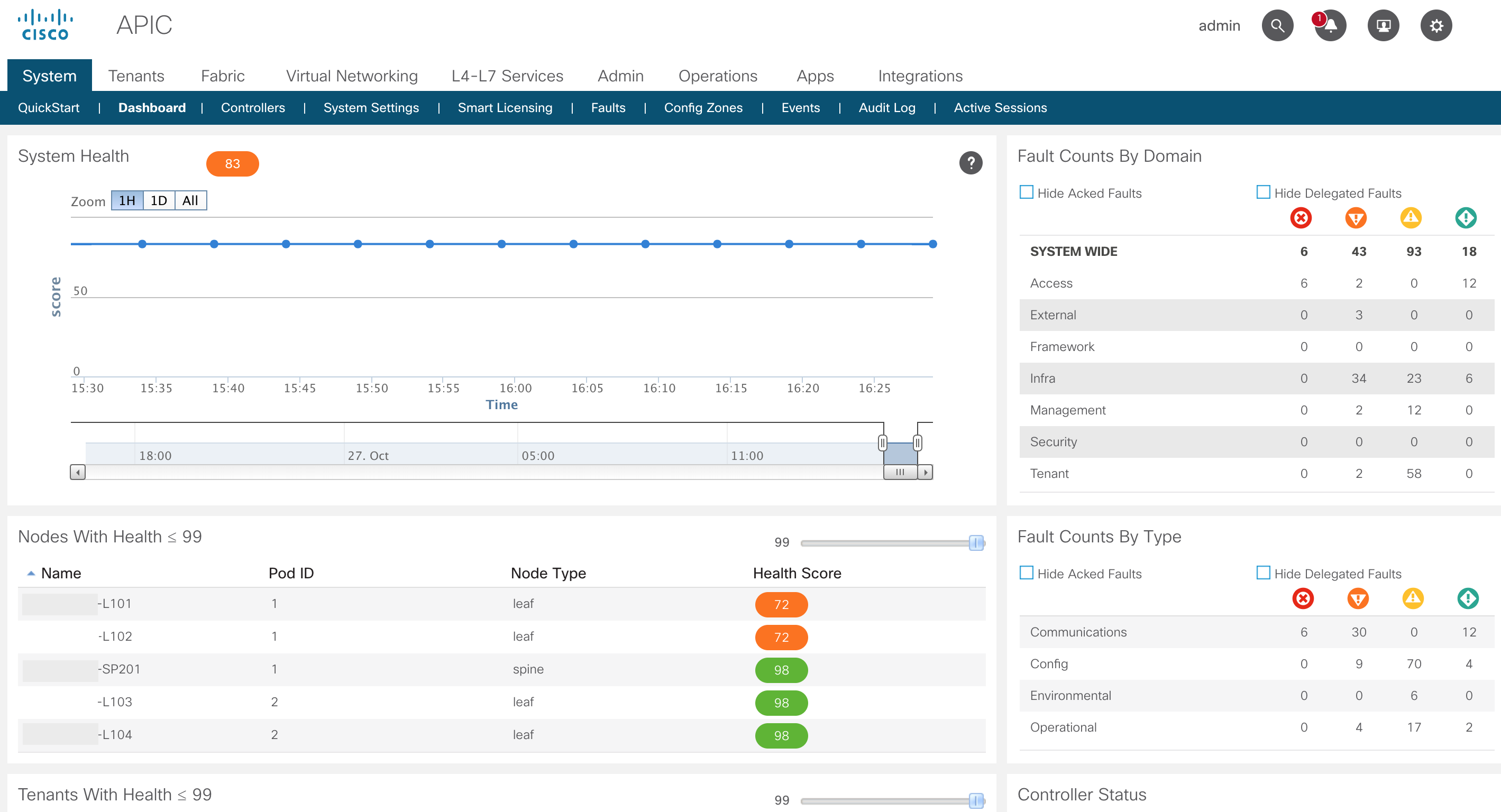
The APIC also monitors the health of the complete fabric and reports on this. An administrator can see the health of the complete fabric in ‘a single pane of glass’.
APICs should never be alone. They come in clusters. ACI uses a database model in which the database is split into a number of parts. These parts are called shards. Each shard will be copied three times and will be distributed along the APICs. Any time two APICs with a copy of a shard is online that part of the database can be edited. This is also called a majority. Because you have two of the three available copies you can edit that part of the database, because the third copy, when it becomes available again will take over the information from the majority. This means that when you have three APICs and they all have a copy of each shard the whole database will be read-only when two of the three APICs go down.
The number of APICs in the cluster depends on the size of the fabric. The number of supported switches differs per version and you would be best of by searching your favorite search engine for the terms “ACI verified scalability guide ”
For version 4.0 you will find that a 3 node cluster supports 80 leaf switches and a 4 or bigger node cluster supports 200 leaf switches. As a shard will not be copied more than three times, a three node cluster is recommended if you don’t need more than 80 leaf switches. If you do you can grow beyond three APICs, but failure of two of them might mean that some parts of the database are writeable and some aren’t. However, there is no way to know which parts will be read-only and which parts will be read-write. When you have five nodes you might even encounter the situation in which three of the APICs are down causing parts of the database to be completely unavailable.
For this last reason, Cisco recommends not to include more than two APICs in a single datacenter if you have a multi-pod setup (more on multi-pod later).
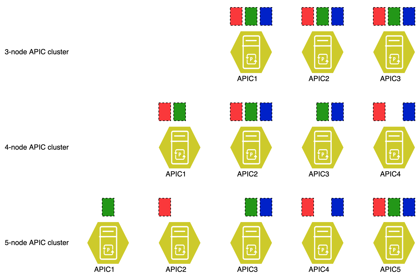
The image displays the problem with five APICs and database sharding. In the image you see three types of clusters. As you can see the red, green and blue database shards are present on all APICs in the 3-node APIC cluster. The 4-node cluster appears to have a decent spread, but when APIC1 and APIC2 go down the database enters a minority state for both red and green shards, but remains in majority for the blue shard. This causes the APIC cluster to be able to edit the data contained in the blue shard, but not the data in the red and green shards. The 5-node cluster makes the effect even more extreme. If in this case APICs 3 through 5 go down (because they are in the same datacenter for example), the blue shard is gone completely. That information is unavailable for the time those APICs are gone. What makes it worse, you can’t (currently) restore the database on APICs 1 and 2.
ACI Topology
When we talk about the ACI topology we actually need to specify which topology we mean. ACI provides an underlay and overlay network. For this explanation we will start with the underlay network.
ACI underlay network
The underlay network is the physical network with all required protocols that make the overlay network work. So what does this underlay network entail? Physically the ACI network is very simple. It’s a Spine-Leaf topology. This is often called a Clos Network. The Wikipedia page however goes into too much detail for this discussion. There are some basic things to know about the ACI topology:
- Every Spine switch must be connected to every Leaf switch
- Every Leaf switch must be connected to every Spine switch (follows from 1.)
- Leaf switches must not connect to Leaf switches and Spine switches must not connect to Spine switches
- Everything that is not a Leaf switch must not be connected to a Spine, but to a Leaf (a few exceptions apply)
The list above form the ground rules for an ACI fabric. However, there are several designs possible and we need to know them all. Some of these designs bend the rules a little.
We’ve got the following designs for ACI:
- Single pod
- Stretched fabric
- Multi-Pod
- Multi-Site
We’ll discuss these designs in more detail in a few minutes, but before we do let’s zoom in a bit more on the underlay itself. As any network engineer knows, just connecting stuff doesn’t make a network work. Something more is needed. Protocols.
The underlay network in ACI is just a regular network. It runs IP (version 4) and uses the ISIS routing protocol. IP runs over ethernet (as can be expected) but there is no broadcast. All links in the network are direct IP links. This means that ACI does not run Spanning Tree in the underlay (or in the overlay for that matter). All links are active an used in an ECMP manner.
The ACI software automates the configuration of the underlay for you. When you bring up a fabric for the first time you have to specify some information (more about this in the chapter about fabric Discovery, which will follow later). Part of this information are the IP addresses ACI will use and the vlan it will use for its infrastructure.
You might ask that if this is an underlay that is automated completely, why don’t they just make up some IP addresses and vlan? The reason is that there are features and topologies imaginable that extend the underlay, making it a routed network into your existing network. This might cause some issues. Cisco recommends using an IP range which isn’t in use anywhere else in the fabric.
This range of IP addresses is called the TEP range and will be requested during staging. The recommended size of the TEP range is a /16, but smaller is allowed for small fabrics. The minimum size depends on the ACI version, but has been /22 for several versions now.
When a switch is discovered by the fabric it will be provisioned with an IP address. (Actually, several of them might be present, depending on the configuration). Below is an example of my lab:
IP Interface Status for VRF "overlay-1"(4)
Interface            Address              Interface Status
eth1/49              unassigned           protocol-up/link-up/admin-up
eth1/49.8            unnumbered           protocol-up/link-up/admin-up
                     (lo0)
eth1/50              unassigned           protocol-down/link-down/admin-up
eth1/51              unassigned           protocol-down/link-down/admin-up
eth1/52              unassigned           protocol-down/link-down/admin-up
eth1/53              unassigned           protocol-down/link-down/admin-up
eth1/54              unassigned           protocol-down/link-down/admin-up
vlan7                10.190.0.30/27       protocol-up/link-up/admin-up
lo0                  10.190.240.34/32     protocol-up/link-up/admin-up
lo1                  10.190.184.67/32     protocol-up/link-up/admin-up
lo1023               10.190.0.32/32       protocol-up/link-up/admin-up
This output shows you some interfaces that are part of the VRF that is used for the underlay. The physical interfaces are all the uplink ports. The logical interfaces are assigned dynamically:
- lo0: Automatically configured during switch discovery. This is the address that will be used as the VTEP. It’s also the address that is used as interface address on the uplink interfaces (using the ip unnumbered command)
- lo1: Assigned to the vPC VTEP. When a switch is configured as part of a vPC pair it will be assigned an additional IP address. This is the vPC VTEP.
- lo1023: This will always be present. This is used when the infrastructure VXLAN is extended out of the fabric. This is used when using the Cisco AVS or AVE virtual switches. The IP address is also called the FTEP
- vlan7: This might differ on each implementation, but it translates to the infra vlan. This vlan interface is used to communicate with the APIC. You can see this vlan will map to the vlan you’ve configured as the infrastructure vlan using the
show vlan extendedcommand. This interface should only be present when something is connected to the LEAF switch using the infrastructure vlan.
There might be more interfaces present depending on the features enabled on the switch and its role.
The funny thing here is that the VRF for the underlay is called overlay-1. This name is automatic and can’t be changed anywhere.
The APICs take care of the configuration of the underlay routing protocols too. The actual underlay uses ISIS to exchange underlay routing information. Anything that is related to the underlay like the location of the VTEP addresses of other switches is exchanged using ISIS. You can verify the existence of the neighbor adjacencies and routes using the show isis commands like in the example below:
NETWORKOUT-POD1-SP101# show isis adjacency vrf overlay-1
IS-IS process: isis_infra VRF:overlay-1
IS-IS adjacency database:
System ID         SNPA            Level  State  Hold Time  Interface
20F0.BE0A.0000     N/A            1      UP     00:00:57   Ethernet1/1.38
22F0.BE0A.0000     N/A            1      UP     00:01:01   Ethernet1/3.37
NETWORKOUT-POD1-SP101#
NETWORKOUT-POD1-SP101# show isis route vrf overlay-1
IS-IS process: isis_infra VRF: overlay-1
IS-IS IPv4 routing table
10.190.0.1/32
    *via 10.190.240.34, eth1/3.37, metric 11
10.190.184.67/32
    *via 10.190.240.34, eth1/3.37, metric 2
    *via 10.190.240.32, eth1/1.38, metric 2
10.190.240.32/32
    *via 10.190.240.32, eth1/1.38, metric 2
10.190.240.34/32
    *via 10.190.240.34, eth1/3.37, metric 2
Another protocol running in the underlay is BGP. BGP is used to exchange external routing information into the fabric. The exact usage of BGP in the fabric will be explained in more detail later when we will discuss L3outs.
NETWORKOUT-POD1-SP101# show bgp vpnv4 unicast summ vrf all
BGP summary information for VRF overlay-1, address family VPNv4 Unicast
BGP router identifier 201.201.201.201, local AS number 65123
BGP table version is 39, VPNv4 Unicast config peers 4, capable peers 3
4 network entries and 4 paths using 832 bytes of memory
BGP attribute entries [4/576], BGP AS path entries [0/0]
BGP community entries [0/0], BGP clusterlist entries [0/0]

Neighbor        V    AS MsgRcvd MsgSent   TblVer  InQ OutQ Up/Down  State/PfxRcd
10.190.240.32   4 65123   43369   43369       39    0    0     4w2d 2
10.190.240.34   4 65123  106641  106641       39    0    0    10w4d 2
202.202.202.202 4 65123   87508   88689       39    0    0     4w2d 0
Single pod fabric
The single pod fabric is the most simple implementation of ACI. This was also the first generation ACI design. It just consisted of several Spine switches and several Leaf switches and they were connected following the aforementioned rules.
Physically it’s very simple as can be seen in the image below.
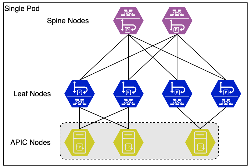
A note on images. I will use a consistent format for all images. This means that the above image is the first image depicting an ACI fabric. Spines are Purple, Leafs are blue (and sometimes green if they have a special function), APICs are yellow and non-ACI devices are red. The icon for each type of device is also different. This first image shows the roles of each icon in text next to it.
Stretched fabric
Pretty soon after the introduction of ACI customers wanted to be able to have their ACI fabric available on two different locations. Whether these were different rooms in the same building or completely different buildings.
Cisco introduced the Stretched Fabric option in ACI 1.0(3). This made the following design possible.
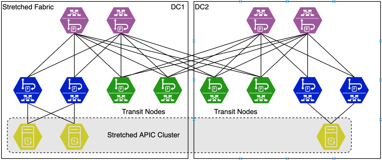
As you can see in the image depicting the stretched fabric, this is the first design breaking the ground rule of connecting all spines to all leafs. Cisco recognized that running fiber between all leafs in a remote location and vice versa was cost prohibitive. So they came up with the idea of Transit Nodes. These were leaf switches that connected to spine switches in the other site. The fabric in this case was still a single fabric.
There are some downsides of the stretched fabric, such as suboptimal traffic flow, but all in all it is still a valid design.
You can use any leaf switch as transit leaf. There are no special requirements for the leafs.
Keep in mind that it is recommended to provide sufficient leaf and spine connections between the two sites to provide redundancy. Failure of a single leaf of spine should not lead to the breaking of the inter site connectivity.
As for the maximum distance between two sites in a stretched fabric design, according to the stretched fabric knowledge base article, a distance of 800Km has been verified. (I personally would not recommend using stretched fabric for those distances). To be able to reach the 800Km distance you would have to use special solutions such as DWDM or MPLS networks to transport the data. However, ACI requires LLDP between devices for discovery to work, so any transport medium must transport LLDP (and therefore be a L2 connection)
A stretched fabric enables flat layer 2 mobility between the sites as each bridge domain is available in both the sites.
We’ll go into more detail of Stretched fabric (and Multi-Pod and Multi-Site) topologies in a later chapter.
Multi-Pod
Multi-Pod is an evolution of the stretched fabric design. A multi-pod fabric is still a kind of stretched fabric. Like a stretched fabric a multi-pod fabric is still managed by a single APIC cluster. The biggest difference between stretched fabric and multi-pod is the scalability of a multi-pod fabric. It can scale to a lot of sites (as of version 3.0, 12 pods are supported). Stretched fabric, in the current release only supports 3 sites. Multi-pod also increases the number of spine and leaf nodes that are supported.
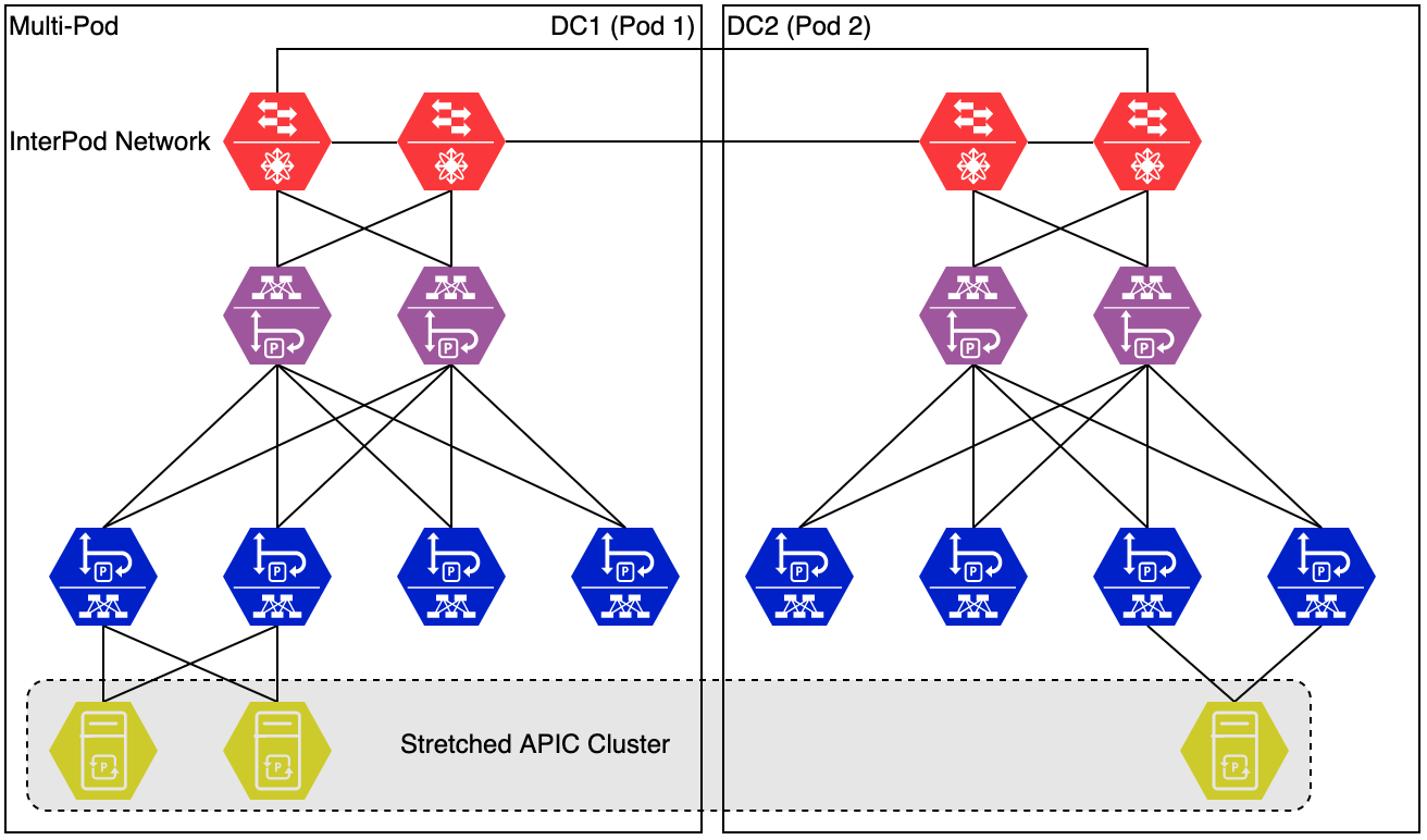
To be able to scale to this size, a multi-pod topology requires a special network between the pods. This is called the InterPod Network (IPN). This IPN is external to the fabric, so won’t be managed by the APIC.
There are some requirements to the IPN, which we will cover in detail later. For now, remember that the IPN must support OSPF and PIM BIDIR.
Multi-site
The multi-site design is yet another design that covers multiple sites. When looking at the image below and comparing it to the multi-pod variant you might not notice a lot of differences in the first place. The Multi-Site architecture looks very similar, but is very different.
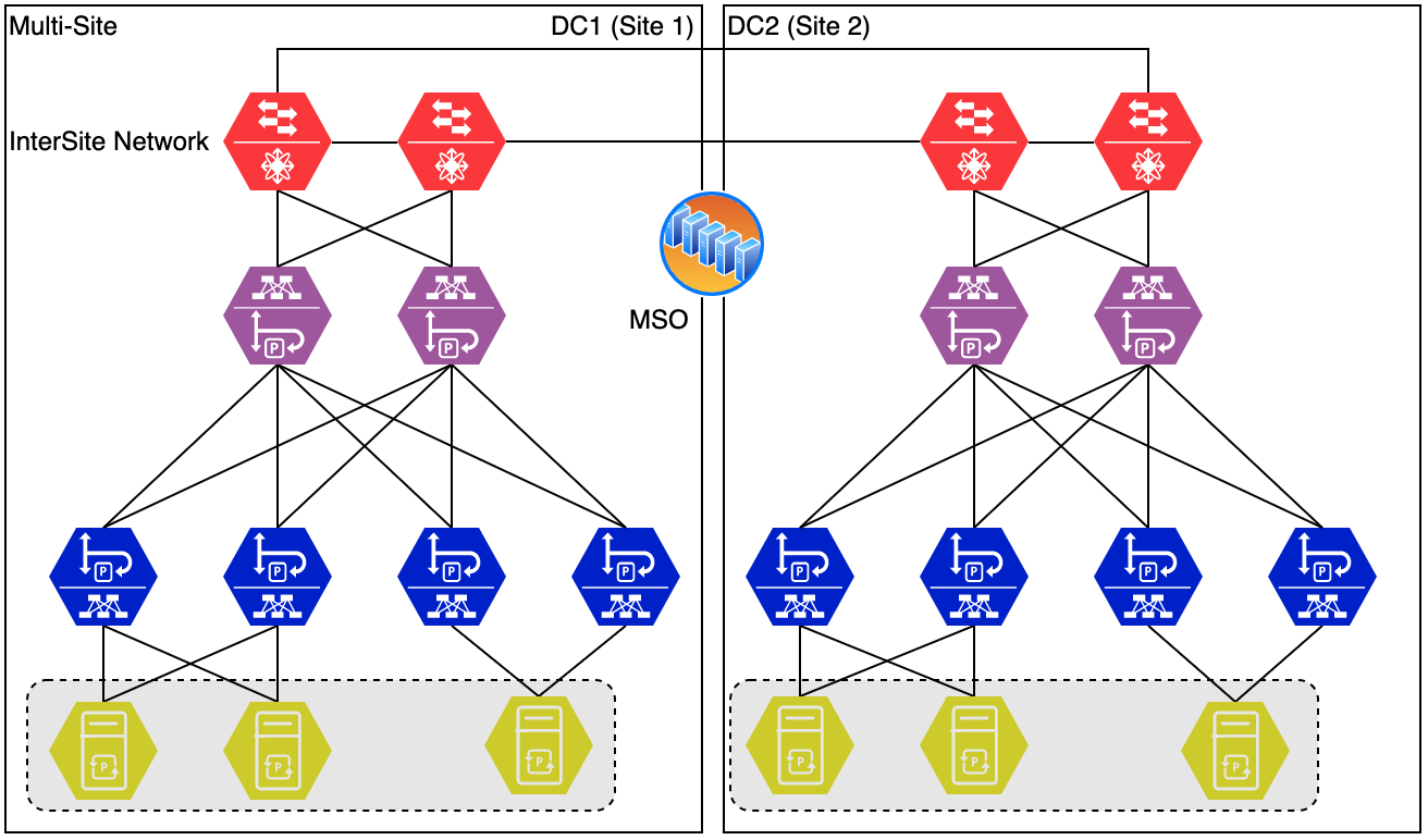
A multi-site fabric consists of multiple separate fabrics. Each fabric has its own APIC cluster. The difference between Multi-Site and just connecting separate ACI fabrics using L3out connectivity is the orchestrator that runs on top of it. This orchestrator is called the Multi-Site Orchestrator (MSO). This enables an administrator to easily set up connectivity between sites and have tenants stretching the sites (even Bridge Domains and EPGs can stretch.)
There will be a whole chapter on these topologies.
Other topologies
As ACI continues to develop different topologies emerge. These will be covered later, but are listed here for completeness:
- Remote Leaf
- vPod
- cPod
- Cloud Only